Low-Pass Filters
Low-pass filters are basically an upgrade from the Averaging filters. If you are not familiar with averaging filter, may be it is a good idea to go through them first.
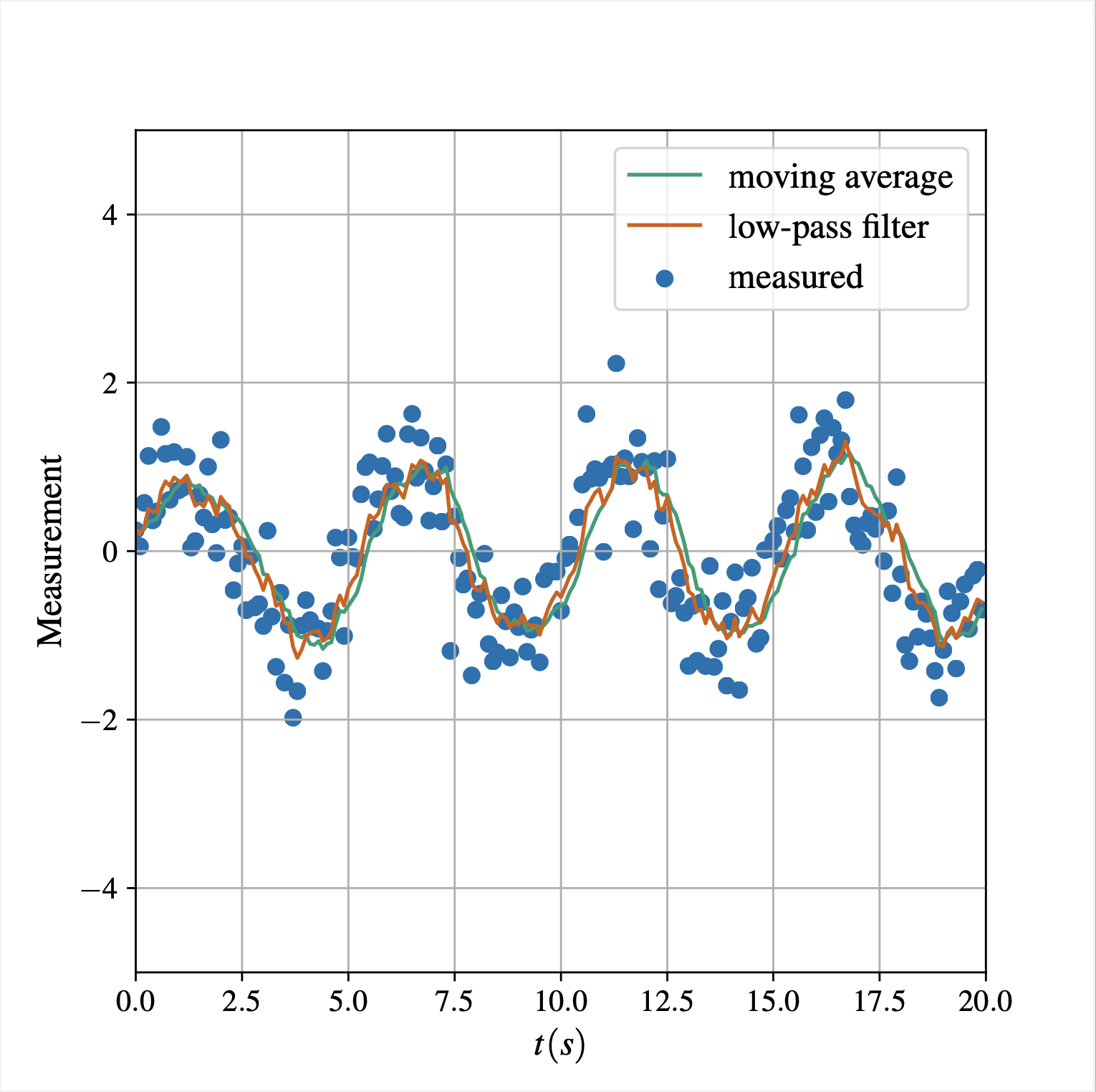
Usually, the noise is in high frequency bands. The low-pass filter is designed to pass-through low frequency signals, while blocking high frequency signals, hence the name “low-pass filter”.
The moving average filter has the same weight for all measurements. However, in reality, the most recent measurements have more to say about the current state. The low-pass filter overcome this by using a heavier weight on the most recent data.
The first order low-pass filter can be written as follows with \(0 < \alpha < 1\).
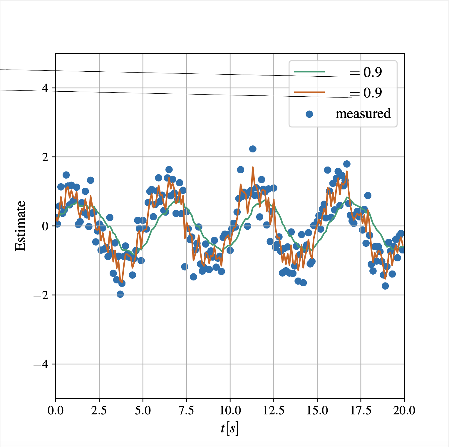
\[x_k = \alpha \cdot x_{k - 1} + (1 - \alpha) \cdot x_k\]This is a bit similar to average filter, but \(\alpha\) can be set arbitrarily. Higher \(\alpha\) (closer to 1) means less noise, but lags, while lower \(\alpha\) (closer to 0) means less lag, but noisy.
The first order low-pass filter in Laplace domain is:
\[\frac{Y(s)}{X(s)} = K \cdot \frac{1}{\tau s + 1}\]Examples
See Also
References
- Kim, P. (2011). Kalman Filter for Beginners: with MATLAB Examples. CreateSpace Independent Publishing Platform