Averaging Filters
Any practical measurement has a some level of noise. To meaningfully utilize such measurements, we need to “filter” these noise levels. This is where filters are useful. There are a few commonly used filters, and this post discusses the most basic ones.
Simple Average Filter
Simple averaging can be one of the simplest form of filtering. Here, all of the measurements are used to calculate their mean value. Assume that the measurement at $k$-th time step is $x_k$. Then, the output of the average filter takes the form:
\[x_k = \frac{x_1 + x_2 + ... + x_k}{k}\]However, you may notice that for this calculation, you need to keep a log of all the measurements so far, starting from $k = 0$. To avoid that, the above expression can be re-arranged as:
\[x_k = \frac{k - 1}{k} \cdot x_{k - 1} + \frac{1}{k} \cdot x_k\]If we let \(\alpha = \frac{k - 1}{k}\), we can further simplify the above expression to:
\[x_k = \alpha \cdot x_{k - 1} + (1 - \alpha) \cdot x_k\]This is referred to as the recursive averaging equation.
Example
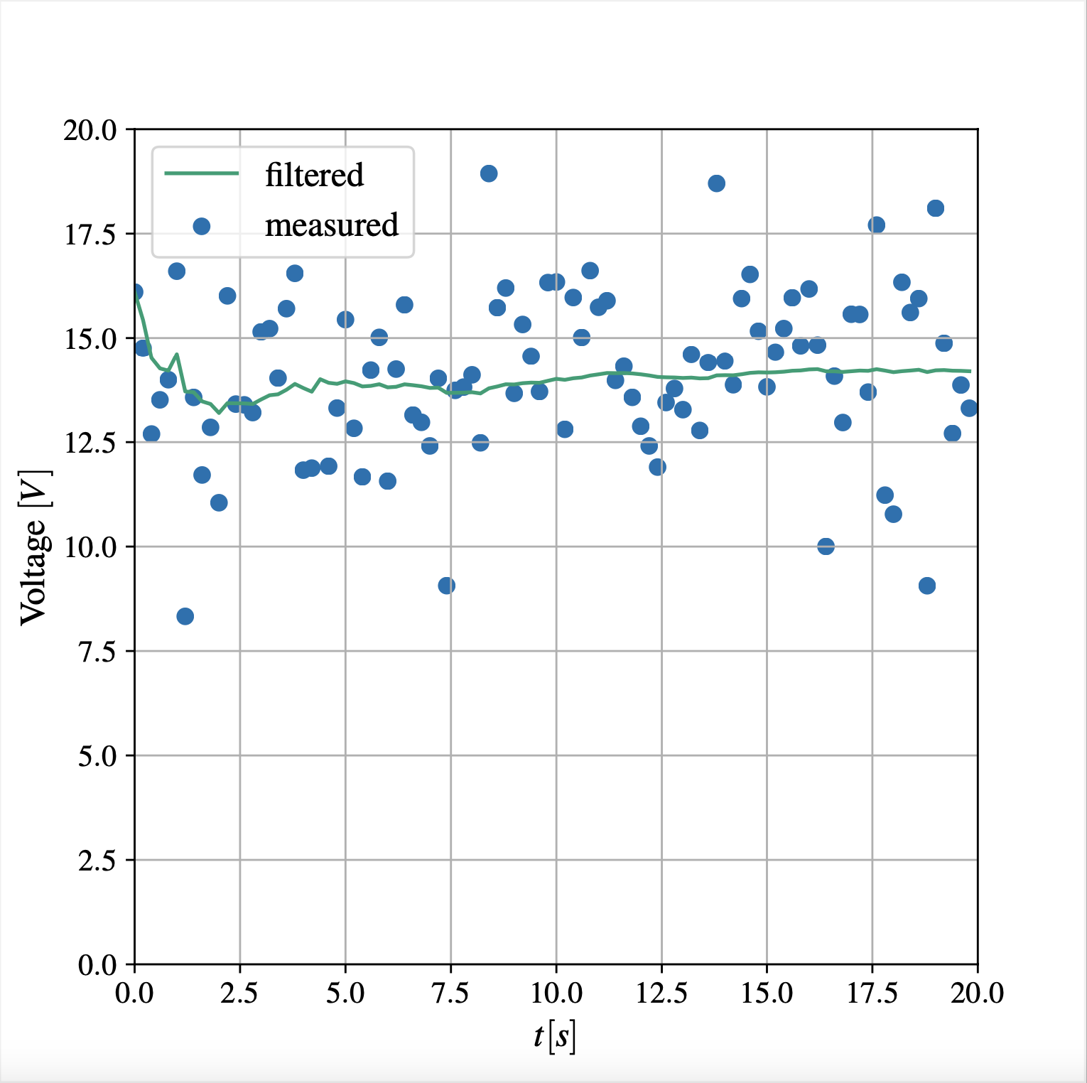
Consider the following example, adopted from the Reference 1 at the bottom of this page. A voltmeter measures a constant voltage of 14 V. The measurement noise is modeled as a white noise of 0 V mean and a standard deviation of 2 V.
Pros and Cons
As shown in the above figure, the value converges to the actual value, even in the presence of large sensor noise. Also, the algorithm is simple and computationally inexpensive.
However, since this averages all past data, the filtered is heavily weighted by them. This works fine for a constant measurement, but if the measured state changes with time, average filter is going to provide seriously lagged output. Check the following section for visualizations.
Moving Average Filter
Moving average filter is similar to the average filter, but only considers the few most recent data sets. This way, the past data does not weigh down the filtered data as much as the averaging filter. The equation for \(n\)-moving average filter:
\[x_k = \frac{x_{k - (n - 1)} + x_{k - (n - 2)} + ... + x_k}{n}\]We can re-arrange this to get a cleaner looking moving average filter equation:
\[x_k = x_{k - 1} + \frac{x_k - x_{k - n}}{n}\]Example
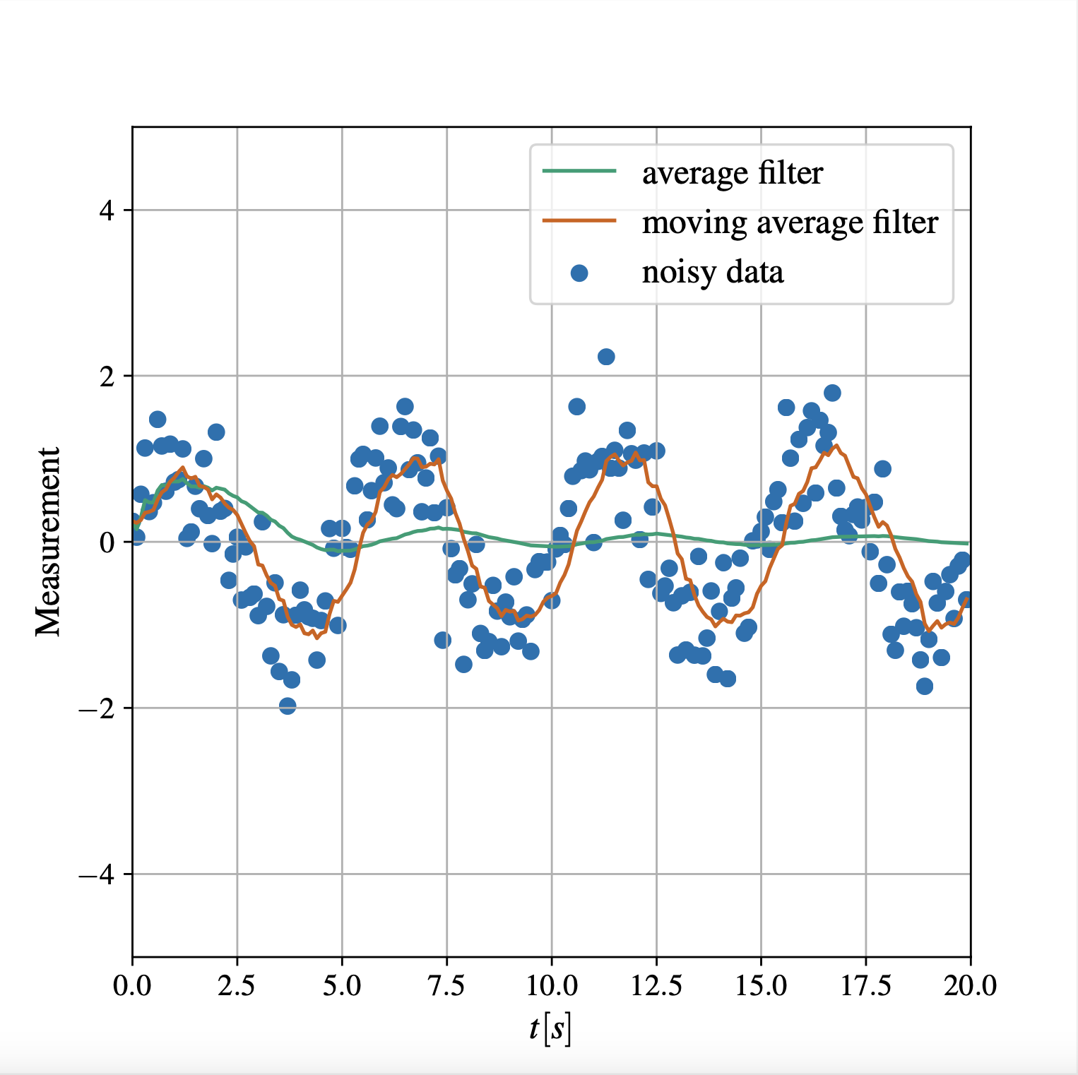
Consider a case where the moving average filter applied to noisy sinusoidal data.
Here, the measured value changes at a faster phase. The averaging filter we discussed in the previous section cannot keep up with the rate of change. However, the moving average filter deal with the situation better, with a slight lag.
It is also important to note that when the number of averaging points increases, it provides a better noise reductions, but increases the delay in responding to the changes.
See Also
References
- Kim, P. (2011). Kalman Filter for Beginners: with MATLAB Examples. CreateSpace Independent Publishing Platform